Model and Estimation

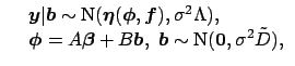
Semi-parametric nonlinear mixed-effects (SNM) models extend current statistical nonlinear models for grouped data in two directions: adding flexibility to a nonlinear mixed-effects model by allowing the mean function to depend on some non-parametric functions, and providing ways to model covariance structure and covariates effects in an SNR model. An SNM model assumes that

$$y_{ij} = \eta(\mbox{\boldmath$\phi$}_{i}, \mbox{\boldmath$f$}; \mbox{\bold... ...$}_{ij}) + \epsilon_{ij}, \,\,\, \, j=1, \cdots, n_{i},\,\,\,\, i=1, \cdots, m,$$ (42)

$$\mbox{\boldmath$\phi$}_{i} = A_i \mbox{\boldmath$\beta$}+ B_i \mbox{\boldmath$b$}_{i},\,\,\, \, \mbox{\boldmath$b$}_{i}\stackrel{iid}{\sim} \mbox{N}({\bf0}, \sigma^{2} D),$$ (43)

where the first-stage model () is the same as a SNR model (), and the second-stage model is the same as one for a nonlinear mixed-effect model. Specifically, $y_{ij}$ is the response of subject $i$ at design point $\mbox{\boldmath$t$}_{ij}$, $\mbox{\boldmath$t$}_{ij}=(t_{1ij},\cdots,t_{dij})$ are independent variables in a general domain ${\cal T}$, $\eta$ is a known function of $\mbox{\boldmath$t$}_{ij}$ which depends on a vector of parameter $\mbox{\boldmath$\phi$}_i=(\phi_{i1},\cdots,\phi_{ir})^T$ and a vector of unknown non-parametric function $\mbox{\boldmath$f$}=(f_1,\cdots,f_q)^T$; random errors $\mbox{\boldmath$\epsilon$}=(\epsilon_{11}, \cdots, \epsilon_{1n_1}, \cdots,\epsilon_{m1},\cdots,\epsilon_{mn_m}) \sim \mbox{N} (0, \sigma^2 \Lambda)$; $\mbox{\boldmath$\beta$}$ is a $p$-vector of fixed effects, $\mbox{\boldmath$b$}_{i}$ is $k$-vector of random effects associated with subject $i$; $A_i$ and $B_i$ are design matrices of sizes $r\times p$ and $r\times k$ for the fixed and random effects respectively. It is assumed that the random effects and random errors are mutually independent. Each function $f_j$ is modeled using an SS ANOVA model ().

Let $n=\sum_{i=1}^m n_i$, $\mbox{\boldmath$y$}_{i}=(y_{i1},\cdots,y_{in_{i}})^{T}$, $\mbox{\boldmath$y$}=(\mbox{\boldmath$y$}_{1}^{T}, \cdots,\mbox{\boldmath$y$}_{m}^{T})^{T}$, $\mbox{\boldmath$\phi$}=(\mbox{\boldmath$\phi$}_{1}^{T}, \cdots, \mbox{\boldmath$\phi$}_{m}^{T})^{T}$, $\mbox{\boldmath$\eta$}_{i}(\mbox{\boldmath$\phi$}_{i}, \mbox{\boldmath$f$})=(\e... ...x{\boldmath$\phi$}_{i}, \mbox{\boldmath$f$}; \mbox{\boldmath$t$}_{in_{i}}))^{T}$, $\mbox{\boldmath$\eta$}(\mbox{\boldmath$\phi$}, \mbox{\boldmath$f$})=(\mbox{\bol... ...mbox{\boldmath$\eta$}_{m}^T(\mbox{\boldmath$\phi$}_m, \mbox{\boldmath$f$}))^{T}$ and $\mbox{\boldmath$b$}=(\mbox{\boldmath$b$}_{1}^{T}, \cdots, \mbox{\boldmath$b$}_{m}^{T})^{T}$. The SNM model () and () can then be written in a matrix form

$$\begin{array}{clcr} &\mbox{\boldmath$y$}\vert\mbox{\boldmath$b$}\... ...\,\, \mbox{\boldmath$b$}\sim \mbox{N}({\bf0}, \sigma^{2}\tilde{D}), \end{array}$$ (44)

where $A=(A_{1}^T, \cdots, A_{m}^T)^T$, $B=\mbox{diag}(B_1, \cdots, B_m)$ and $\tilde{D}=\mbox{diag}(D, \cdots, D)$. In the following we assume that $\Lambda$ and $D$ depend on an unknown parameter vector $\mbox{\boldmath$\tau$}$.

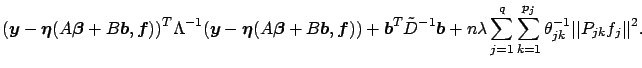
For fixed $\mbox{\boldmath$\tau$}$ and $\sigma^2$, we estimate $\mbox{\boldmath$\beta$}$, $\mbox{\boldmath$f$}$, $\mbox{\boldmath$b$}$, $\mbox{\boldmath$\tau$}$ as the minimizers of the following double penalized log-likelihood

$$(\mbox{\boldmath$y$}-\mbox{\boldmath$\eta$}(A \mbox{\boldmath$\be... ...um_{j=1}^q \sum_{k=1}^{p_j} \theta_{jk}^{-1} \vert\vert P_{jk}f_j\vert\vert^2 .$$ (45)

Denote $\tilde{\mbox{\boldmath$\beta$}}$, $\tilde{\mbox{\boldmath$f$}}$ and $\tilde{\mbox{\boldmath$b$}}$ as solutions to (). Let $\tilde{Z}=(\partial\mbox{\boldmath$\eta$}(A\mbox{\boldmath$\beta$}+B\mbox{\bold... ...rtial\mbox{\boldmath$b$}^{T})_{\mbox{\boldmath$b$}=\tilde{\mbox{\boldmath$b$}}}$, and $\tilde{V}=\Lambda+\tilde{Z} \tilde{D} \tilde{Z}^T$. We estimate $\mbox{\boldmath$\tau$}$ and $\sigma^2$ as minimizers of the approximate profile log-likelihood

$$\log \vert\sigma^2\tilde{V}\vert +\sigma^{-2} (\mbox{\boldmath$y$... ...ath$b$}},\tilde{\mbox{\boldmath$f$}}) +\tilde{Z} \tilde{\mbox{\boldmath$b$}}) .$$ (46)

Since $\mbox{\boldmath$f$}$ may interact with $\mbox{\boldmath$\beta$}$ and $\mbox{\boldmath$b$}$ in a complicated way, we have to use iterative procedures to solve () and (). We proposed two procedures in Ke and Wang (2001) for the case when $\eta$ is linear in $\mbox{\boldmath$f$}$. It is not difficult to extend these procedures to the general case. In the following we describe the extension of Procedure 1 in Ke and Wang (2001).

Procedure 1: estimate $\mbox{\boldmath$f$}$, $\mbox{\boldmath$\beta$}$, $\mbox{\boldmath$b$}$, $\mbox{\boldmath$\tau$}$ and $\sigma^2$ iteratively using the following three steps:

(a) given the current estimates of $\mbox{\boldmath$\beta$}$, $\mbox{\boldmath$b$}$ and $\mbox{\boldmath$\tau$}$, update $\mbox{\boldmath$f$}$ by solving ();

(b) given the current estimates of $\mbox{\boldmath$f$}$ and $\mbox{\boldmath$\tau$}$, update $\mbox{\boldmath$\beta$}$ and $\mbox{\boldmath$b$}$ by solving ();

(c) given the current estimates of $\mbox{\boldmath$f$}$, $\mbox{\boldmath$\beta$}$ and $\mbox{\boldmath$b$}$, update $\mbox{\boldmath$\tau$}$ and $\sigma^2$ by solving ().

Note that step (b) corresponds to the pseudo-data step and step (c) corresponds to part of the LME step in Lindstrom and Bates (1990). Thus the nlme can be used to accomplish (b) and (c). In step (a) () is reduced to () after certain transformations. Then depending on if $\eta$ is linear in $\mbox{\boldmath$f$}$, the ssr or nnr function can be used to update $\mbox{\boldmath$f$}$. We choose smoothing parameters using a data-adaptive criterion such as GCV, GML or UBR at each iteration.

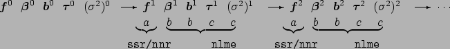
To minimize () we need to alternate between steps (a) and (b) until convergence. Our simulations indicate that one iteration is usually enough. Figure shows the flow chart of Procedure 1 if we alternate (a) and (b) only once. Step (a) can be solved by ssr or nnr. It is easy to see that steps (b) and (c) are equivalent to fitting a NLMM with $\mbox{\boldmath$f$}$ fixed at the current estimate using the same methods proposed in Lindstrom and Bates (1990). Therefore these two steps can be combined and solved by S program nlme (Pinheiro and Bates, 2000). Figure suggests an obvious iterative algorithm by calling nnr and nlme alternately. It is not difficult to use other options in our implementation. For example, we may alternate steps (a) and (b) several times before proceeding to step (c). In our studies these approaches usually gave the same results. For details about the estimation methods and procedures, see Ke and Wang (2001).

Figure: Flow chart of Procedure 1. The first row shows the order in which parameters are updated. The second row indicates the corresponding step for each parameter. The third row indicates that step (a) can be solved by ssr or nnr and steps (b) and (c) can be combined and solved by nlme.

Approximate Bayesian confidence intervals can be constructed for $\mbox{\boldmath$f$}$ (Ke and Wang, 2001).