Potassium Measurements on Dogs

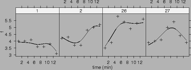
36 dogs were assigned to four groups: control, extrinsic cardiac denervation three weeks prior to coronary occlusion, extrinsic cardiac denervation immediately prior to coronary occlusion, and bilateral thoratic sympathectomy and stellectomy three weeks prior to coronary occlusion. Coronary sinus potassium concentrations were measured on each dog every two minutes from 1 to 13 minutes after occlusion (Grizzle and Allen, 1969). Observations are shown in Figure .

Figure: Plots of responses of each dog over time. Solid lines link within group average responses at each time point.

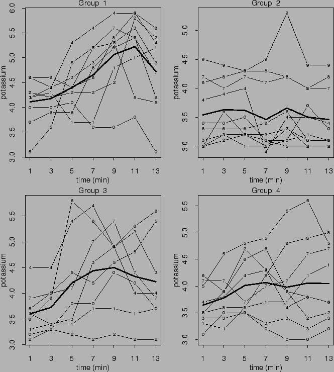We are interested in (i) estimating the group (treatment) effects; (ii) estimating the population mean concentration as functions of time; and (iii) predicting response over time for each dog. There are two categorical covariates group and dog and a continuous covariate time. We code the group factor as 1 to 4, and the observed dog factor as 1 to 36. We transform the time variable into [0,1]. We treat group and time are fixed factors. From the design, the dog factor is nested within the group factor. Therefore we treat dog as a random factor. For group $k$, denote ${\cal B}_k$ as the population from which the dogs in group $k$ were drawn and ${\cal P}_k$ as the sampling distribution. Assume the following model

$$y_{kwj} = f(k,w,t_j) + \epsilon_{kwj};~~~~k=1,\cdots,4; ~~w \in {\cal B}_k; ~~t_j \in [0,1] ,$$

where $y_{kwj}$ is the observed potassium concentration at time $t_j$ of dog $w$ in the population ${\cal B}_k$, $f(k,w,t_j)$ is the ``true'' concentration at time $t_j$ of dog $w$ in the population ${\cal B}_k$, and $\epsilon_{kwj}$'s are random errors. $f(k,w,t_j)$ is a function defined on $\{ \{1 \} \otimes {\cal B}_1, \{2 \} \otimes {\cal B}_2, \{3 \} \otimes {\cal B}_3, \{4 \} \otimes {\cal B}_4 \} \otimes [0,1]$. Note that $f(k,w,j)$ is a random variable since $w$ is a random sample from ${\cal B}_k$. What we observe are realizations of this ``true'' mean function plus random errors. We use label $i$ to denote dogs we actually observe.

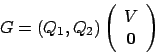
Suppose that we want to model the time factor using a cubic spline, and shrink both the group and dog factors toward constants. We define the following four projection operators:

$$\begin{eqnarray*} P_2f &=& \int_{{\cal B}_k} f(k,w,t) d{\cal P}_k(w), \\ P_1f &... ..._4f &=& [\int_0^1 (\partial f(k,w,t) / \partial t) dt] (t-0.5) . \end{eqnarray*}$$

Then we have the following SS ANOVA decomposition

$$f$$

$$= [P_1+(P_2-P_1)+(I-P_2)][P_3+P_4+(I-P_3-P_4)] f$$

$$= P_1P_3 f+P_1P_4 f+P_1(I-P_3-P_4) f$$

$$+(P_2-P_1)P_3 f + (P_2-P_1)P_4 f+ (P_2-P_1) (I-P_3-P_4) f$$

$$+(I-P_2)P_3 f + (I-P_2)P_4 f + (I-P_2)(I-P_3-P_4) f$$

$$= \mu + \beta (t-0.5) + s_1(t)$$

$$+ \xi_k + \delta_k (t-0.5) + s_2(k,t)$$

$$+ \alpha_{w(k)} + \gamma_{w(k)} (t-0.5) + s_3(k,w,t),$$ (78)

where $\mu$ is a constant, $\beta (t-0.5)$ is the linear main effect of time, $s_1(t)$ is the smooth main effect of time, $\xi_k$ is the main effect of group, $\delta_k (t-0.5)$ is the linear interaction between time and group, $s_2(k,t)$ is the smooth interaction between time and group, $\alpha_{w(k)}$ is the main effect of dog, $\gamma_{w(k)} (t-0.5)$ is the linear interaction between time and dog, and $s_3(k,w,t)$ is the smooth interaction between time and dog. We can calculate the main effect of time as $\beta (t-0.5)+s_1(t)$, the interaction between time and group as $\delta_k (t-0.5) + s_2(k,t)$, and the interaction between time and dog as $\gamma_{w(k)} (t-0.5) + s_3(k,w,t)$. The first six terms are fixed effects. The last three terms are random effects since they depend on the random variable $w$. Depending on time only, the first three terms represent the mean curve for all dogs. The middle three terms measure the departure of a particular group from the population mean curve. The last three terms measure the departure of a particular dog from the mean curve of a population from which the dog was chosen.

Based on the SS ANOVA decomposition (), we will fit the following three models.

Model 1 includes the first seven terms in (). It has a different population mean curve for each group plus a random intercept for each dog. We assume that $\alpha_{i} \stackrel{iid}{\sim} \mbox{N} (0,\sigma^2_a)$, $\epsilon_{kij} \stackrel{iid}{\sim} \mbox{N}(0,\sigma^2)$, and they are mutually independent.

Model 2 includes the first eight terms in (). It has a different population mean curve for each group plus a random intercept and a random slope for each dog. We assume that $(\alpha_i,\gamma_i) \stackrel{iid}{\sim} \mbox{N} ((0,0), \mbox{diag}(\sigma^2_1,\sigma^2_2))$, $\epsilon_{kij} \stackrel{iid}{\sim} \mbox{N}(0,\sigma^2)$, and they are mutually independent.

Model 3 includes all nine terms in (). It has a different population mean curve for each group plus a random intercept, a random slope and a smooth random effect for each dog. We assume that $(\alpha_i,\gamma_i) \stackrel{iid}{\sim} \mbox{N} ((0,0), \mbox{diag}(\sigma^2_1,\sigma^2_2))$, $s_3(k,i,t)$'s are stochastic processes which are independent between dogs with mean zero and covariance function $\sigma_3^2 [k_2(s)k_2(t)-k_4(s-t)]$, $\epsilon_{kij} \stackrel{iid}{\sim} \mbox{N}(0,\sigma^2)$, and they are mutually independent.

Now we show how to fit these three models using slm. Notice that the fixed effects, $s_1(t)$, $\xi_k$, $\delta_k (t-0.5)$ and $s_2(k,t)$ are penalized. Model 1 and Model 2 can be fitted easily as follows.

> dog.fit1 <- slm(y~time, rk=list(cubic(time), shrink1(group), 
                  rk.prod(kron(time-.5), shrink1(group)),
                  rk.prod(cubic(time), shrink1(group))), 
                  random=list(dog=~1), data=dog.dat)
> dog.fit1
Semi-parametric linear mixed-effects model fit by REML
  Model: y ~ time 
  Data: dog 
  Log-restricted-likelihood: -180.4784

Fixed: y ~ time 
(Intercept)        time 
  3.8716387   0.4339031 

Random effects:
 Formula: ~1 | dog
        (Intercept)  Residual
StdDev:   0.4980483 0.3924432


GML estimate(s) of smoothing parameter(s) : 0.0002334736 0.0034086209 
                                            0.0038452499 0.0002049233 
Equivalent Degrees of Freedom (DF):  13.00377 
Estimate of sigma:  0.3924432 


> dog.fit2 <- update(dog.fit1, random=list(dog=~time))
> dog.fit2
Semi-parametric linear mixed-effects model fit by REML
  Model: y ~ time 
  Data: dog.dat 
  Log-restricted-likelihood: -166.4478

Fixed: y ~ time 
 (Intercept)      time 
    3.876712 0.4196789

Random effects:
 Formula:  ~ time | dog
 Structure: General positive-definite
               StdDev   Corr 
(Intercept) 0.4188372 (Inter
       time 0.5593078 0.025 
   Residual 0.3403214       

GML estimate(s) of smoothing parameter(s) : 
1.674736e-04 3.286466e-03 5.778379e-03 8.944005e-05 
Equivalent Degrees of Freedom (DF):  13.83273 
Estimate of sigma:  0.3403214

To fit Model 3, we need to find a way to specify the smooth (non-parametric) random effect $s_3$. Let $\mbox{\boldmath$t$}=(t_1,\cdots,t_7)^T$, $u_i(\mbox{\boldmath$t$})=(s_3(k,i,t_1),\cdots,s_3(k,i,t_7))^T$ and $\mbox{\boldmath$u$}=(\mbox{\boldmath$u$}_1^T,\cdots,\mbox{\boldmath$u$}_{36}^T)^T$. Then $u_i(\mbox{\boldmath$t$}) \stackrel{iid}{\sim} \mbox{N} (0,\sigma_3^2 D)$, where $D$ is the RK of a cubic spline evaluated at the design points $\mbox{\boldmath$t$}$. Let $D = H H^T$ be the Cholesky decomposition of $D$, $\tilde{D}=\mbox{diag}(D, \cdots, D)$, and $G=\mbox{diag} (H,\cdots,H)$. Then $G G^T=\tilde{D}$. We can write $\mbox{\boldmath$u$}=G \mbox{\boldmath$b$}$, where $\mbox{\boldmath$b$}\sim \mbox{N} (0,\sigma_3^2 I)$. Then we can specify the random effects $\mbox{\boldmath$u$}$ using the matrix $G$.

> D <- cubic(dog.dat$time[1:7])
> H <- chol.new(D)
> G <- kronecker(diag(36), H)
> dog.dat$all <- rep(1,36*7)
> dog.fit3 <- update(dog.fit2, random=list(all=pdIdent(~G-1), dog=~time)) 
> dog.fit3
Semi-parametric linear mixed-effects model fit by REML
  Model: y ~ time 
  Data: dog.dat 
  Log-restricted-likelihood: -150.0885

Fixed: y ~ time 
 (Intercept)      time 
    3.885269 0.4046573

Random effects:
 Formula:  ~ G - 1 | all
 Structure: Multiple of an Identity
...

 Formula:  ~ time | dog %in% all
 Structure: General positive-definite
               StdDev   Corr 
(Intercept) 0.4671536 (Inter
       time 0.5716811 -0.083
   Residual 0.2383432       


GML estimate(s) of smoothing parameter(s) : 
8.775590e-05 1.560998e-03 3.346731e-03 2.870384e-05 
Equivalent Degrees of Freedom (DF):  15.37699 
Estimate of sigma:  0.2383432

We could use the anova function for linear mixed-effects models to compare these three fits.

> anova(dog.fit1$lme.obj, dog.fit2$lme.obj, dog.fit3$lme.obj)
                 Model df      AIC      BIC    logLik   Test  L.Ratio p-value 
dog.fit1$lme.obj     1  8 376.9590 405.1307 -180.4795                        
dog.fit2$lme.obj     2 10 352.8955 388.1101 -166.4478 1 vs 2 28.06346  <.0001
dog.fit3$lme.obj     3 11 322.1771 360.9131 -150.0885 2 vs 3 32.71845  <.0001

So Model 3 is more favorable. We can calculate estimates of the population mean curves for four groups as follows.

> dog.grid <- data.frame(time=rep(seq(0,1,len=50),4), 
                         group=as.factor(rep(1:4,rep(50,4))))
> e.dog.fit3 <- intervals(dog.fit3, newdata=dog.grid, terms=rep(1,6))

Figure plots these mean curves and their 95% confidence intervals.

Figure: Estimates of the population mean response curve as a function of time with their 95% confidence intervals. Circles are within group average responses. Solid lines are estimates. Dotted lines are 95% confidence intervals.

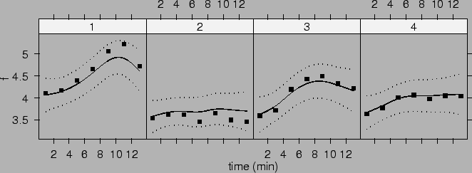We have shrunk the effects of group factor toward constants. That is, we have penalized the group main effect $\xi_k$ and the linear time-group interaction $\delta_k (t-0.5)$ in the SS ANOVA decomposition (). From Figure we can see that the estimated population mean curve for group 2 are biased upward, while the estimated population mean curves for group 1 is biased downward. This is because responses from group 2 are smaller while responses from group 1 are larger than those from groups 3 and 4. Thus their estimates are pulled towards the overall mean. Shrinkage estimates in this case may not be advantageous since group only has four levels. One may want to leave $\xi_k$ and $\delta_k (t-0.5)$ terms unpenalized to reduce biases. We can re-write the fixed effects in () as

$$f_k(t) \stackrel{def}{=} \mu + \beta (t-0.5) + s_1(t) + \xi_k + \delta_k (t-0.5) + s_2(k,t)$$

$$= [\mu+ \xi_k]+[\beta (t-0.5)+ \delta_k (t-0.5)]+[ s_1(t)+ s_2(k,t)]$$

$$= \tilde{\xi}_k + \tilde{\delta_k} (t-0.5)+\tilde{s}_2(k,t).$$ (79)

$f_k(t)$ is the population mean curve for group $k$. Assume $f_k \in W_2([0,1])$. Define penalty as $\int_0^1 (f_k^{\prime\prime}(t))^2 dt=\vert\vert\tilde{s}_2(k,t)\vert\vert^2$. Then the constant term $\tilde{\xi}_k$ and the linear term $\tilde{\delta_k} (t-0.5)$ are not penalized. Note that this form of penalty was used in Wang (1998b). We can refit Model 1, Model 2 and Model 3 under this new form of penalty as follows.

> dog.fit4 <- slm(y~group*time, rk=list(rk.prod(cubic(time), kron(group==1)),
                                        rk.prod(cubic(time), kron(group==2)),
                                        rk.prod(cubic(time), kron(group==3)),
                                        rk.prod(cubic(time), kron(group==4))), 
                  random=list(dog=~1), data=dog.dat)
> dog.fit4
Semi-parametric linear mixed-effects model fit by REML
  Model: y ~ group * time 
  Data: dog 
  Log-restricted-likelihood: -173.0538

Fixed: y ~ group * time 
(Intercept)      group2      group3      group4        time group2:time 
 4.30592658 -0.70377899 -0.45507981 -0.54411601  0.70494987 -0.80352151 
group3:time group4:time 
-0.02604081 -0.33005253 

Random effects:
 Formula: ~1 | dog
        (Intercept)  Residual
StdDev:   0.4986658 0.3880457


GML estimate(s) of smoothing parameter(s) : 2.470589e-05 1.290422e+00 
                                            7.737418e-05 8.136673e-04 
Equivalent Degrees of Freedom (DF):  13.05131 
Estimate of sigma:  0.3880457 

> dog.fit5 <- update(dog.fit4, random=list(dog=~time))
> dog.fit5
Semi-parametric linear mixed-effects model fit by REML
  Model: y ~ group * time 
  Data: dog 
  Log-restricted-likelihood: -158.7129

Fixed: y ~ group * time 
(Intercept)      group2      group3      group4        time group2:time 
 4.31780496 -0.71566053 -0.46280282 -0.55513686  0.68418592 -0.78275742 
group3:time group4:time 
-0.01217737 -0.30620677 

Random effects:
 Formula: ~time | dog
 Structure: General positive-definite, Log-Cholesky parametrization
            StdDev    Corr  
(Intercept) 0.4225180 (Intr)
time        0.5536860 -0.005
Residual    0.3367037       


GML estimate(s) of smoothing parameter(s) : 1.714698e-05 3.894053e+00 
                                            5.640272e-05 4.988060e-04 
Equivalent Degrees of Freedom (DF):  13.74553 
Estimate of sigma:  0.3367037 

> dog.fit6 <- update(dog.fit5, random=list(all=pdIdent(~G-1), dog=~time)) 
> dog.fit6
Semi-parametric linear mixed-effects model fit by REML
  Model: y ~ group * time 
  Data: dog 
  Log-restricted-likelihood: -142.3147

Fixed: y ~ group * time 
(Intercept)      group2      group3      group4        time group2:time 
 4.33679882 -0.72758015 -0.47372184 -0.57605073  0.65150749 -0.75063284 
group3:time group4:time 
 0.00427347 -0.26053905 

Random effects:
 Formula:  ~ G - 1 | all
...

 Formula: ~time | dog %in% all
 Structure: General positive-definite, Log-Cholesky parametrization
            StdDev    Corr  
(Intercept) 0.4688705 (Intr)
time        0.5665381 -0.104
Residual    0.2394261       


GML estimate(s) of smoothing parameter(s) : 8.175602e-06 1.567092e+00 
                                            3.081125e-05 1.289556e-01 
Equivalent Degrees of Freedom (DF):  13.43655 
Estimate of sigma:  0.2394261 

> anova(dog.fit4$lme.obj, dog.fit5$lme.obj, dog.fit6$lme.obj)
                 Model df      AIC      BIC    logLik   Test  L.Ratio p-value
dog.fit4$lme.obj     1 14 374.1076 423.0680 -173.0538                        
dog.fit5$lme.obj     2 16 349.4257 405.3804 -158.7129 1 vs 2 28.68192  <.0001
dog.fit6$lme.obj     3 17 318.6295 378.0814 -142.3148 2 vs 3 32.79624  <.0001

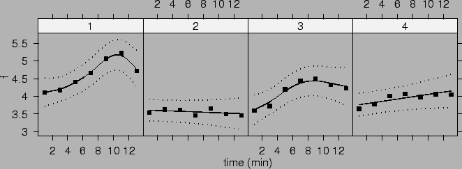
We note that the estimates are similar to, but not exactly the same as, those calculated by SAS proc mixed in Wang (1998b). The differences may be caused by different starting values and/or numerical procedures. We calculate estimates of the population mean curves for four groups as before.

> e.dog.fit6 <- intervals(dog.fit6, newdata=dog.grid, terms=rep(1,12))

Figure plots these mean curves and their 95% confidence intervals.

Figure: Estimates of the population mean response curve as a function of time with their 95% confidence intervals. Circles are within group average responses. Solid lines are estimates. Dotted lines are 95% confidence intervals.

We now show how to calculate predictions for dogs. Prediction for dog $i$ in group $k$ on a point $t$ can be computed as $\hat{\xi}_k + \hat{\delta}_k (t-0.5) + \hat{s}_2(k,t) + \hat{\alpha}_i + \hat{\gamma}_i (t-0.5) + \hat{s}_3(k,i,t)$. Prediction of the fixed effects can be computed using the prediction.slm function. $\hat{\alpha}_i$ and $\hat{\gamma}_i$ are provided in the estimates of the random effects. Thus we only need to compute $\hat{s}_3(k,i,t)$. Suppose that we want to predict $s_3$ for dog $i$ in group $k$ on a vector of points $\mbox{\boldmath$z$}_i=(z_{i1},\cdots,z_{ig_i})^T$. Let $u_i(\mbox{\boldmath$z$}_i)=(s_3(k,i,z_{i1}),\cdots,s_3(k,i,z_{ig_i}))^T$,

$$R_i=\mbox{Cov} ( u_i(\mbox{\boldmath$z$}_i), u_i(\mbox{\boldmath$t$})) = {\{ R_1(z_{ik},t_j) \}_{k=1}^{g_i}}_{j=1}^7,$$

where $R_1(z,t)=k_2(z)k_2(t)-k_4(z-t)$. Let $\mbox{\boldmath$z$}=(\mbox{\boldmath$z$}_1^T,\cdots,\mbox{\boldmath$z$}_{36}^T)^T$, $R=\mbox{diag} (R_1,\cdots,R_{36})$ and $\hat{\mbox{\boldmath$u$}}$ be the prediction of $\mbox{\boldmath$u$}$. We then can compute the prediction for all dogs as

$$\hat{u}(\mbox{\boldmath$z$})=R \tilde{D}^{-1} \hat{\mbox{\boldmath$u$}} .$$

However the smallest eigen-value of $D$ is close to zero, thus $\tilde{D}^{-1}$ cannot be calculated precisely. We will use an alternative approach which does not require inverting $D$. Denote the estimate of $\mbox{\boldmath$b$}$ as $\hat{\mbox{\boldmath$b$}}$. If we can find a vector $\mbox{\boldmath$c$}$ (need not to be unique) such that

$$G^T \mbox{\boldmath$c$}= \hat{\mbox{\boldmath$b$}}.$$ (80)

Then

$$\hat{u}(\mbox{\boldmath$z$})=R \tilde{D}^{-1} \hat{\mbox{\bo... ...e{D}^{-1} (G G^T) \mbox{\boldmath$c$} = R \mbox{\boldmath$c$}.$$

So the task now is to solve (). Let

$$G=(Q_1,Q_2) \left( \begin{array}{c} V \\ {\bf0} \end{array}\right)$$

be the QR decomposition of $G$. We consider $\mbox{\boldmath$c$}$ in the space spanned by $Q_1$: $\mbox{\boldmath$c$}=Q_1\mbox{\boldmath$\alpha$}$. Then from (), $\mbox{\boldmath$\alpha$}=V^{-T} \hat{\mbox{\boldmath$b$}}$. Thus $\mbox{\boldmath$c$}=Q_1V^{-T} \hat{\mbox{\boldmath$b$}}$ is a solution to (). This approach also applies to the situation when $D$ is singular. In the following we calculate predictions for all 36 dogs on a set of grid points.

> dog.grid2 <- data.frame(time=rep(seq(0,1,len=50),36),
                          dog=rep(1:36,rep(50,36)))
> R <- kronecker(diag(36),cubic(dog.grid2$time[1:50],dog.dat$time[1:7]))	
> b <- as.vector(dog.fit6$lme.obj$coef$random$all)
> G.qr <- qr(G)
> c.coef <- qr.Q(G.qr)%*%solve(t(qr.R(G.qr)))%*%b
> tmp1 <- c(rep(e.dog.fit6$fit[dog.grid$group==1],9),
            rep(e.dog.fit6$fit[dog.grid$group==2],10),
            rep(e.dog.fit6$fit[dog.grid$group==3],8),
            rep(e.dog.fit6$fit[dog.grid$group==4],9))
> tmp2 <- as.vector(rep(dog.fit6$lme.obj$coef$random$dog[,1],rep(50,36)))
> tmp3 <- as.vector(kronecker(dog.fit6$lme.obj$coef$random$dog[,2],
                              dog.grid2$time[1:50]))	
> u.new <- as.vector(R%*%c.coef)
> p.dog.fit6 <- tmp1+tmp2+tmp3+u.new

Predictions for dogs 1, 2, 26 and 27 are shown in Figure .

Figure: Plots of predictions for dogs 1, 2, 26 and 27. Circles are observations. Solid lines are predictions.

Observations close in time from the same dog may be correlated. In the following we fit a first-order autoregressive structure for random errors within each dog.

> dog.fit7 <- update(dog.fit6, cor=corAR1(form=~1|all/dog))
> dog.fit7
  Model: y ~ group * time 
  Data: dog 
  Log-restricted-likelihood: -132.6711

Fixed: y ~ group * time 
 (Intercept)       group2       group3       group4         time  group2:time 
 4.343695660 -0.760617887 -0.483550117 -0.620851406  0.629970047 -0.715780104 
 group3:time  group4:time 
 0.008927178 -0.239117441 

Random effects:
 Formula:  ~ G - 1 | all
 Structure: Multiple of an Identity
...

 Formula: ~time | dog %in% all
 Structure: General positive-definite, Log-Cholesky parametrization
            StdDev    Corr  
(Intercept) 0.2779298 (Intr)
time        0.2909205 0.991 
Residual    0.4456182       

Correlation structure of class corAR1 representing
      Phi 
0.6359198 

GML estimate(s) of smoothing parameter(s) : 2.921150e-05 1.954848e+06 
                                            1.098781e-04 1.893688e+01 
Equivalent Degrees of Freedom (DF):  11.63503 
Estimate of sigma:  0.4030084

By convention in nlme, model dog.fit7 may also be fitted as

dog.fit8 <- update(dog.fit6, cor=corAR1(form=~1))