Rock Data

The rock data in Venables and Ripley (1998) contains measurements on four cross-sections of each of 12 oil-bearing rocks. The aim is to predict permeability (perm) from three other measurements: the total area (area), total perimeter (peri) and a measure of ``roundness'' of the pores in the rock cross-section (shape). Venables and Ripley (1998) fitted this data set with a projection pursuit (PP) regression model. Here we show how to use the snr function to fit the following PP regression model

$$\log (\mbox{\tt perm}) = f(\alpha_1 \times \mbox{\tt area} + \alpha_2 \times \mbox{\tt peri} + \times \alpha_3 \mbox{\tt shape}) + \epsilon,$$ (81)

where $\alpha_1^2+\alpha_2^2+\alpha_3^2=1$ and $\alpha_3>0$ for identifiability.

We first fit model () using the R function ppr as in Venables and Ripley (1998). Then we fit the same model using snr with initial values from the ppr fit. We use a TPS with $d=1$ and $m=2$ to model $f$. We made the following transformations: dividing area and peri by 10000, and taking the natural logarithm of perm.

> data(rock)
> attach(rock)
> area1 <- area/10000; peri1 <- peri/10000
> rock.ppr <- ppr(log(perm) ~ area1 + peri1 + shape,
                  data=rock, nterms=1, max.terms=5)
> summary(rock.ppr)
Call:
ppr(formula = log(perm) ~ area1 + peri1 + shape, rock.Rdata = rock,
    nterms = 1, max.terms = 5)

Goodness of fit:
  1 terms   2 terms   3 terms   4 terms   5 terms
19.590843  8.737806  5.289517  4.745799  4.490378

Projection direction vectors:
       area1        peri1        shape
 0.347565455 -0.937641311  0.005198698

Coefficients of ridge terms:
[1] 1.495419

> rock.snr <- snr(log(perm) ~ f(a1*area1+a2*peri1+sqrt(1-a1^2-a2^2)*shape),
                  func=f(u)~list(~u,tp(u)),
                  params=list(a1+a2~1),
                  start=list(params=c(.34,-.94)))
> rock.snr
Semi-parametric Nonlinear Regression Model Fit
 Model: log(perm) ~ f(a1 * area1 + a2 * peri1 + sqrt(1 - a1^2 - a2^2) *      shape)

 Log-likelihood: -50.04593

Coefficients:
        a1         a2
 0.3449282 -0.9386264

Smoothing spline:
 GCV estimate(s) of smoothing parameter(s): 1.249731e-06
 Equivalent Degrees of Freedom (DF):  4.144281

Residual standard error: 0.770572
Number of Observations: 48


Converged after 5 iterations

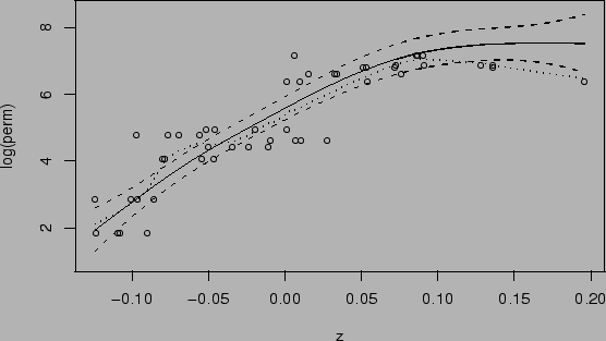
> a <- seq(min(z),max(z),len=50)
> rock.snr.ci <- intervals(rock.snr,newdata=data.frame(u=a))
> rock.ppr.p <- predict(rock.ppr)

snr converged after 5 iterations. Let $z=\hat{\alpha_1} \times \mbox{\tt area1} + \hat{\alpha_2} \times \mbox{\tt peri1} + \sqrt{1-\hat{\alpha_1}^2-\hat{\alpha_2}^2} \times \mbox{\tt shape}$. In Figure , against the $z$ values, we plot the observations as circles, the fitted curve $f$ from rock.snr as the solid line with 95% Bayesian confidence intervals as the dotted lines, and the shape of the fitted curve $f$ from rock.ppr as the dashed line. The fitted curves from snr and ppr have different shapes.

Figure: Plot of perm on logarithm scale vs $z$ values as circles. The solid line is the fitted curve from rock.snr. Two dotted lines are its 95% Bayesian confidence intervals. The dashed line represents the shape of the fitted curve from rock.ppr.