CO$_2$ Uptake Data

This dataset comes from a study of cold tolerance of a $C_4$ grass species, Echinochloa crus-galli, described in Potvin et al. (1990) and Pinheiro and Bates (2000). A total of twelve four-week-old plants were used in the study. There were two types of plants: six from Quebec and six from Mississippi. Two treatments, nonchilling and chilling, were assigned to three plants of each type. Nonchilled plants were kept at $26^o$C and chilled plants were subject to 14 hours of chilling at $7^o$C. After 10 hours of recovery at $20^o$C, CO$_2$ uptake rates (in $\mu mol/m^2s$) were measured for each plant at seven concentrations of ambient CO$_2$ in increasing, consecutive order. Plots of observations are shown in Figure as circles. The objective of the experiment was to evaluate the effect of plant type and chilling treatment on the CO$_2$ uptake.

Figure: Plots of the data and fitted curves. Circles are observations. Solid lines represent SNM model fits from co2.fit2. Dotted lines represent NLMM fits from co2.fit1. In the strip name for each plot, ``Q'' indicates Quebec, ``M'' Mississippi, ``c'' chilled, ``n'' nonchilled, and ``1'', ``2'', ``3'' the replicate numbers.

Pinheiro and Bates (2000) gave detailed analyses of this dataset based on NLMMs using their software nlme. They reached the following model:

$$\mbox{\tt uptake}_{ij} = e^{\phi_{1i}} \{1-e^{-e^{\phi_{2i}} (\mbox{\tt conc}_j-\phi_{3i})}\}+\epsilon_{ij}, \ \ i=1, \cdots,12,\ \ j=1, \cdots, 7,$$

$$\phi_{1i} = \beta_{11}+\beta_{12}\mbox{\tt Type}+\beta_{13} \mbox{\tt Treatment}+\beta_{14}\mbox{\tt Treatment:Type} + b_i,$$

$$\phi_{2i} = \beta_{21} ,$$

$$\phi_{3i} = \beta_{31}+\beta_{32}\mbox{\tt Type}+\beta_{33} \mbox{\tt Treatment}+\beta_{34}\mbox{\tt Treatment:Type} ,$$ (82)

where $\mbox{\tt uptake}_{ij}$ denotes the CO$_2$ uptake rate of plant $i$ at CO$_2$ ambient concentration $\mbox{\tt conc}_j$; Type equals 0 for plants from Quebec and 1 for plants from Mississippi, Treatment equals 0 for chilled plants and 1 for control plants; $e^{\phi_{1i}}$, $e^{\phi_{2i}}$ and $\phi_{3i}$ denote respectively the asymptotic uptake rate, the uptake growth rate, and the maximum ambient CO$_2$ concentration at which no uptake is verified for plant $i$; random effects $b_i \stackrel{iid}{\sim}N({\bf0}, \sigma_b^2)$; and random errors $\epsilon_{ij}\stackrel{iid}{\sim}N(0, \sigma^2)$. Note that we used exponential transformations to enforce the positivity constraints.

> options(contrasts=rep("contr.treatment", 2))	
> co2.fit1 <- nlme(uptake~exp(a1)*(1-exp(-exp(a2)*(conc-a3))), 
                   fixed=list(a1+a2~Type*Treatment,a3~1), 
                   random=a1~1, groups=~Plant, data=CO2,
                   start=c(log(30),0,0,0,log(0.01),0,0,0,50))
> co2.fit1
Nonlinear mixed-effects model fit by maximum likelihood
  Model: uptake ~ exp(a1) * (1 - exp(-exp(a2) * (conc - a3))) 
 Data: CO2 
       AIC      BIC    logLik
  393.2869 420.0259 -185.6434

Random effects:
 Formula: a1 ~ 1 | Plant
        a1.(Intercept) Residual
StdDev:     0.08221494 1.857658

Fixed effects: list(a1 + a2 ~ Type * Treatment, a3 ~ 1) 
                                       Value Std.Error DF   t-value p-value
a1.(Intercept)                       3.73338  0.052536 64  71.06301  <.0001
a1.TypeMississippi                  -0.29080  0.075535 64  -3.84990  0.0003
a1.Treatmentchilled                 -0.07274  0.074633 64  -0.97459  0.3334
a1.TypeMississippi:Treatmentchilled -0.51321  0.109733 64  -4.67688  <.0001
a2.(Intercept)                      -4.57570  0.086116 64 -53.13387  <.0001
a2.TypeMississippi                  -0.09635  0.103950 64  -0.92687  0.3575
a2.Treatmentchilled                 -0.17048  0.091377 64  -1.86565  0.0667
a2.TypeMississippi:Treatmentchilled  0.70555  0.205851 64   3.42748  0.0011
a3                                  49.98833  4.576255 64  10.92341  <.0001
...

Fits of model () are plotted in Figure as dotted lines. Based on model (), one may conclude that the CO2 uptake is higher for plants from Quebec and that chilling, in general, results in lower uptake, and its effect on Mississippi plants is much larger than on Quebec plants. These conclusions are comparable to the results in Potvin et al. (1990).

We aim to use this dataset to demonstrate how to fit SNM models with covariates, and how to check if an NLMM is appropriate. As an extension of (), we fit the following SNM model

$$\mbox{\tt uptake}_{ij} = e^{\phi_{1i}} f(e^{\phi_{2i}}(\mbox{\tt conc}_j-\phi_{3i}))+\epsilon_{ij}, \ \ i=1, \cdots,12,\ \ j=1, \cdots, 7,$$

$$\phi_{1i} = \beta_{12}\mbox{\tt Type}+\beta_{13} \mbox{\tt Treatment}+\beta_{14}\mbox{\tt Treatment:Type} + b_i,$$

$$\phi_{2i} = \beta_{21} ,$$

$$\phi_{3i} = \beta_{31}+\beta_{32}\mbox{\tt Type}+\beta_{33} \mbox{\tt Treatment}+\beta_{34}\mbox{\tt Treatment:Type} ,$$ (83)

where $f\in W_2([0, T])$ for some fixed $T>0$ and the second stage model is paralleled to (). In order to test if the parametric model () is appropriate, we construct the following $L$-spline to model $f$. The hypothesis is $H_0$: $f\in span\{1-e^{-t}\}$. Let $L= D + D^2$, where $D^j$ denotes the $j$th derivative operator. The kernel space of $L$ is ${\cal H}_1=span\{1, e^{-t}\}$. Define a linear operator ${\cal B}: W_{2}[0, T]\rightarrow {\cal R}^{2}$ such that ${\cal B}f=(f(0), f'(0))$. Let ${\cal H}_{2}=ker{\cal B}$. Define inner products on ${\cal H}_{1}, {\cal H}_{2}$, and $W_{2}[0, T]$ as $<f, g>_{1}=({\cal B}f)^{T}({\cal B}g)$, $<f, g>_{2}=\int_{0}^{T}(Lf)(Lg)dt$ and $<f, g>=<f, g>_{1}+ <f, g>_{2}$. Then it is easy to check that $W_{2}[0, T]={\cal H}_{1}\oplus {\cal H}_{2}$. The reproducing kernel of ${\cal H}_{2}$ is given in ().

Note that $\beta_{11}$ in () is excluded from () to make $f$ free of constraint on the vertical scale. We need the side conditions that $f(0)=0$ and $f(t)\ne 0$ for $t\ne 0$ to separate $\beta_{31}$ from $f$. The first condition reduces ${\cal H}_1$ to ${\cal H}_1=\mbox{span}\{1-e^{-t}\}$ and is satisfied by all functions in ${\cal H}_2$. We do not enforce the second condition because it is satisfied by all reasonable estimates. Thus the null space for $f$ becomes ${\cal H}_1^0=\mbox{span}\{1- e^{-t}\}$ and the model space is ${\cal H}_1^0\oplus {\cal H}_2$. The penalty is still $J(f)=\int (Lf)^2$.

With the initial values chosen from the NLMM fit, our program converged after 5 iterations.

> M <- model.matrix(~Type*Treatment, data=CO2)[,-1]
> co2.fit2 <- snm(uptake~exp(a1)*f(exp(a2)*(conc-a3)),
                func=f(u)~list(~I(1-exp(-u))-1,lspline(u, type="exp")),
                fixed=list(a1~M-1,a3~1,a2~Type*Treatment),
                random=list(a1~1), group=~Plant, verbose=T,
                start=co2.fit1$coe$fixed[c(2:4,9,5:8)], data=CO2)
> summary(co2.fit2)
Semi-parametric Nonlinear Mixed Effects Model fit
  Model: uptake ~ exp(a1) * f(exp(a2) * (conc - a3)) 
  Data: CO2 

       AIC     BIC    logLik
  406.4864 441.625 -188.3760

Random effects:
 Formula: a1 ~ 1 | Plant
        a1.(Intercept) Residual
StdDev:     0.09304172 1.816200

Fixed effects: list(a1 ~ M - 1, a3 ~ 1, a2 ~ Type * Treatment) 
                                        Value Std.Error DF   t-value p-value
a1.MTypeMississippi                  -0.28569  0.055952 65  -5.10591  <.0001
a1.MTreatmentchilled                 -0.07212  0.054741 65  -1.31739  0.1923
a1.MTypeMississippi:Treatmentchilled -0.54879  0.099184 65  -5.53309  <.0001
a3                                   50.67565  4.226094 65  11.99113  <.0001
a2.(Intercept)                       -4.56698  0.085130 65 -53.64708  <.0001
a2.TypeMississippi                   -0.12162  0.098575 65  -1.23377  0.2217
a2.Treatmentchilled                  -0.16161  0.087009 65  -1.85740  0.0678
a2.TypeMississippi:Treatmentchilled   0.81924  0.211587 65   3.87187  0.0003
...
GCV estimate(s) of smoothing parameter(s): 1.864811 
Equivalent Degrees of Freedom (DF):  4.867178 

Converged after 5 iterations

Fits of model () are plotted in Figure as solid lines. Since the data set is small, different initial values may lead to different estimates. However, the overall fits are similar. We also fitted models with AR(1) within-subject correlations and covariate effects on $\phi_3$. None of these models improve fits significantly. The estimates are comparable to the nonlinear fits and the conclusion is similar to that based on ().

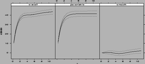
To check if the parametric NLMM () is appropriate, we calculated approximate posterior means and variances using the function intervals. Then we plotted the estimated $f$ (overall), its projection onto ${\cal H}_1^0$ (the parametric part) and ${\cal H}_2$ (the smooth part) in Figure .

> co2.grid2 <- data.frame(u=seq(0.3, 11, len=50))
> co2.ci <- intervals(co2.fit2, newdata=co2.grid2,
                    terms=matrix(c(1,1,1,0,0,1), ncol=2,byrow=T))
> plot.bCI(co2.ci,x=co2.grid2$u,layout=c(3,1),
           type.name=c("overall","parametric","smooth"))

Figure: The overall fit of the common curve (left), its projection onto ${\cal H}_1^0$ (center) and ${\cal H}_2$ (right). Solid lines are fitted values. Dash lines are approximate 95% Bayesian confidence limits.

The zero line is inside the Bayesian confidence intervals for the projection onto ${\cal H}_2$ (smooth component) which suggests that the parametric NLME model ( is adequate.

For $L$-splines, Heckman and Ramsay (2000) showed that selecting the right form of penalty function via a differential operator $L$ can reduce the bias. An $L$-spline allows us to incorporate prior knowledge on the main features of $f$ into the penalty. Usually the form of $L$ is known with coefficients depending on some unknown parameters. Heckman and Ramsay (2000) proposed several methods to estimate these parameters. When the whole model can be written in the form of an SNM model as in this example, our methods can also be used to estimate the penalty. Our approach is the same as the PL (penalized likelihood) approach in Heckman and Ramsay (2000). They commented that the PL method is ``philosophically appealing''. However it is also ``time-consuming'' because a grid search was used. Our method estimates the coefficients in $L$ and the functions $f$ iteratively, thus making it less computationally intensive. In addition, we allow these coefficients to depend on covariates.