Core Body Temperature Data

Circadian rhythms have become a topic of intensive research during the last 40 years. Often the period is fixed as 24 hours due to the entrainment. However, for situations such as when individuals are denied exposure to zeitgebers or are living on irregular sleep/wake schedule, the period of the rhythm must be estimated from data. Several methods such as spectral analysis, autocorrelation, Enright's periodgram and linear regression of onset have been proposed in literature (Arendt et al., 1989; Refinetti, 1993). The first three methods require equidistant samples and the last method requires a marker for the onset of activity. All four methods requres several cycles of observations. Our method illustrated below, under the assumption that the shape of circadian rhythm remains unchanged, can be used for iregular design with few cycles.

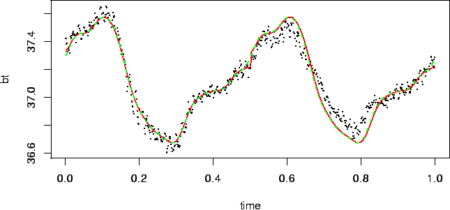
This dataset is taken from a study on mood disorders. We thank Daniel Buysse, MD, and Hernando Ombao, PhD, from the University of Pittsburgh for permission to use part of the data. For several healthy and depressed subjects, core body temperature (bt) is measured over time every 5 minutes for 48 hours. Each subject is put into an isolated room free of time cues. We only use data from one subject and scale time variable into $[0,1]$. Measurements of this subject are shown in Figure . The goal was to investigate possible effects of mode disorder on the biological rhythms. For other physiological measurements, it is known that biological rhythms exist. They are controlled by the internal clock with a period close to 25 hours. We will assume that biological rhythms exist for core body temperature with a similar period. Then the 48 hour observations contain at least one period. We need to estimate the period and the shape function for each subject. The common practice of fitting a sinusoidal function to each subject may not be appropriate (Wang and Brown, 1996). We demonstrate how to use SNR models to fit such data for further analyses. See Hall et al. (2001) for another interesting example and discussions on identifiability.

Figure: Points are observations. Solid red line is the fit from model (). Dotted green line is the fit from model ().

We consider the following model

$$\mbox{\tt bt}_i=f(\mbox{\tt time}_i- \alpha \times \mbox{int}(\frac{\mbox{\tt time}_i}{\alpha}))+\epsilon_i,$$ (84)

where $f$ is a periodic function on $[0, \alpha]$, $\alpha >0$ is the unknown period, and the $\mbox{int}(x)$ returns the integer part of $x$. We assume an AR(1) correlation structure for random errors $\epsilon_i$'s. Because the period is not unique, we define $\alpha$ as the smallest period to make $f$ identifiable. It is evident that the period is close to 24 hours. Thus we use $\alpha=0.5$ as the initial value. To relax the positive constraint, we reparametrize $\alpha$ as $a^2$ in the following program. We used the GML method to select the smoothing parameter since the GCV under-smoothes in this case.

> cbt.fit1 <- snr(bt~f(time-a**2*floor(time/a**2)),
                func=f(u)~list(~1, periodic(u)), 
                params=list(a~1), data=cbt, spar="m",
                start=list(params=c(sqrt(.5))), cor=corAR1())
> cbt.fit1
Semi-parametric Nonlinear Regression Model Fit
 Model: bt ~ f(time - a^2 * floor(time/a^2)) 
 Data: cbt
 Log-likelihood: 1141.090

Coefficients:
        a 
0.7094294 

Correlation Structure: AR(1)
 Formula: ~1 
 Parameter estimate(s):
      Phi 
0.8456162 
Smoothing spline:
 GML estimate(s) of smoothing parameter(s): 6.161782e-08 
 Equivalent Degrees of Freedom (DF):  21.72078 

Residual standard error: 0.06496144 
Number of Observations: 576 

Converged after 4 iterations

> p.cbt.fit1 <- predict(cbt.fit1)

We can also fit an equivalent model

$$\mbox{\tt bt}_i=g(\beta \times \mbox{\tt time}_i) + \epsilon_i,$$ (85)

where $g$ is an unknown periodic function with period $1$, and $\beta > 0$ is unknown scale parameter. Letting $f(t)=g(\beta t)$, it is easy to check that models () and () are equivalent with $\alpha=1/\beta$. We can fit model () with initial value $\beta=2$ by

> cbt.fit2 <- snr(bt~f(a**2*time), func=f(u)~list(~1, periodic(u)), 
                params=list(a~1), data=cbt, spar="m",
                start=list(params=c(sqrt(2))), cor=corAR1())
> cbt.fit2
Semi-parametric Nonlinear Regression Model Fit
 Model: bt ~ f(a^2 * time) 
 Data: cbt
 Log-likelihood: 1143.045

Coefficients:
       a 
1.412535 

Correlation Structure: AR(1)
 Formula: ~1 
 Parameter estimate(s):
      Phi 
0.8471175 
Smoothing spline:
 GML estimate(s) of smoothing parameter(s): 4.377812e-07 
 Equivalent Degrees of Freedom (DF):  21.38732 

Residual standard error: 0.0649923 
Number of Observations: 576 

Converged after 4 iterations

> p.cbt.fit2 <- predict(cbt.fit2)

Fits from these two models are shown in Figure . They are very close. Both models suggest high auto-correlation. The estimate of $\beta$ is $\hat{\beta}=1.412535^2=1.995255$. $1/1.995255=0.501189$, close to $\hat{\alpha}=.709^2=0.5032901$. The estimated period based on models () and () are 24.15792 and 24.05707 hours respectively.