Wisconsin Epidemiological Study of Diabetic Retinopathy

Wisconsin Epidemiological Study of Diabetic Retinopathy (WESDR) is an epidemiological study of a cohort of diabetic patients receiving their medical care in an 11-county area in Southern Wisconsin. Detailed descriptions of the data can be found in Klein et al. (1988). A number of medical, demographic, ocular and other covariates were recorded at the baseline and later examinations along with a retinopathy score for each eye. As in Wahba et al. (1995), we investigate how progression of diabetic retinopathy at the first follow-up depends on the following covariates: dur (duration of diabetes at baseline), gly (glycosylated hemoglobin, a measure of hyperglycemia), and bmi (body mass index = weight in kg/(height in m)$^2$). As in Wahba et al $(1994)$, we chose a subgroup of the younger onset consisting of 669 subjects with no or non-proliferative retinopathy at the baseline. See Wahba et al. (1995) for details of this data set.

We use this data set to illustrate how to fit smoothing spline models for non-Gaussian data. Firstly, we fit a simple cubic spline

$$\mbox{logit} P(\mbox{\tt prg}=1~\vert~\mbox{\tt bmi})=f(\mbox{\tt bmi}),$$

where $f\in W_2([0,1])$.

> wesdr.fit1<- ssr(prg~bmi, rk=cubic(bmi), data=wesdr, family="binary", 
                   scale=T, spar="u", varht=1)
> summary(wesdr.fit1)
...

Coefficients (d):
(Intercept)         bmi 
  -1.286666    1.793480 

UBR estimate(s) of smoothing parameter(s) : 8.793603e-06 
Equivalent Degrees of Freedom (DF):  6.036309 
Estimate of sigma:  1 

> grid <- data.frame(bmi=seq(min(wesdr$bmi),max(wesdr$bmi),len=100))  
> p.wesdr.fit1 <- predict(wesdr.fit1, grid)

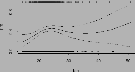
Figure shows the fitted probability function and its 95% Bayesian confidence intervals based on wesdr.fit1.

Figure: Points are observations. Solid line is fitted probability function. Dotted lines are 95% Bayesian confidence intervals.

Wahba et al $(1994)$ reached the following model

$$\mbox{logit} P(\mbox{\tt prg}=1~ \vert~ \mbox{\tt dur}, \mbox{\tt gly}, \mbox{\tt bmi}) = \mu + \alpha*\mbox{\tt gly} + \beta * \mbox{\tt dur} + \gamma * \mbox{\tt bmi} + s_1(\mbox{\tt dur}) + s_2(\mbox{\tt bmi})$$

$$+ ls_{12}(\mbox{\tt dur},\mbox{\tt bmi})+ sl_{12}(\mbox{\tt dur},\mbox{\tt bmi}) + ss_{12}(\mbox{\tt dur},\mbox{\tt bmi}).$$ (77)

The ssr function and related utility functions can be used for model-building. We omit the details and fit () directly.

 
wesdr.fit2<- update(wesdr.fit1, prg~dur+gly+bmi+I(dur*bmi), 
    rk=list(cubic(dur), cubic(bmi), rk.prod(kron(dur), cubic(bmi)),
    rk.prod(kron(bmi), cubic(dur)), rk.prod(cubic(dur), cubic(bmi))))
> summary(wesdr.fit2)
... 
Coefficients (d):
 (Intercept)          dur          gly          bmi I(dur * bmi) 
  -6.1810142   -2.5728071    0.3864040    0.1401764   11.2939414 

UBR estimate(s) of smoothing parameter(s) : 2.653578e+00 3.982479e+00 2.941409e+05 3.086313e+05 8.194281e-02 
Equivalent Degrees of Freedom (DF):  11.19937 
Estimate of sigma:  1 
> grid <- expand.grid(dur=seq(min(wesdr$dur),max(wesdr$dur),len=40),
	              bmi=seq(min(wesdr$bmi),max(wesdr$bmi),len=40),
	              gly=median(wesdr$gly))
> p.wesdr.fit2 <- predict(wesdr.fit2, grid)

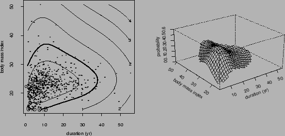
Figure reproduce Figure 6.1 in Wahba et al (1994).

Figure: Left: data and contours of constant posterior standard deviation. Right: estimated probability of progression as a function of durand bmi for gly fixed at its median.